Part 2 ANOVA Basics
As alluded to in Part 1 of this tutorial, we use ANOVA to make decisions about the relationships among means. Typically we do this when we have more than two treatment groups. This is because we could simply use a two-sample t-test to compare two (independent) groups. The power of ANOVA is that we can compare more than two means. For example, let us look at the InsectSprays data set in R (Beall 1942). This simple data set provides counts of insects treated with 6 different insecticides.
First, let us consider the components of this experiment and its design:
Treatment Structure
Factor: Insecticide (spray)
Level: 6 levels (A, B, C, D, E, F)
Design Structure
Experimental Unit: A plot of insects
Randomization Method: Completely randomized design (CRD)
Replication: 12 replicates per type of insecticide (spray)
Response Variable
- Number of insects counted in a plot after application of insecticide
The design structure above warrants some additional discussion. Firstly, the experimental unit is defined as the unit that the treatment is applied. The randomization method of CRD communicates that the experimental units were randomly assigned to each treatment. In this case, insect plots were randomly assigned one of the 6 sprays. Random assignment equalizes the extraneous sources of variability in comparison of the treatment groups. This enables cause and effect conclusions to be drawn from the experiment, protecting against extra variation in the response variable from becoming confounding variables. For example, we might assume that the insects in this study have genetic variation which would make some insects more or less susceptible to certain sprays- CRD makes sure this isn’t the reason a plot responds a certain way to one of the 6 sprays. Lastly, replication is important because it serves to distribute extraneous variation in the response equally, giving us a reasonably equal variance within all treatment groups.
With the preliminaries out of the way, let us now explore the InsectSprays data:
insects <- InsectSprays

insects %>%
  group_by(spray) %>%
  summarise(mean = mean(count), `std dev` = sd(count))
## `summarise()` ungrouping output (override with `.groups` argument)## # A tibble: 6 x 3
## spray mean `std dev`
## <fct> <dbl> <dbl>
## 1 A 14.5 4.72
## 2 B 15.3 4.27
## 3 C 2.08 1.98
## 4 D 4.92 2.50
## 5 E 3.5 1.73
## 6 F 16.7 6.21
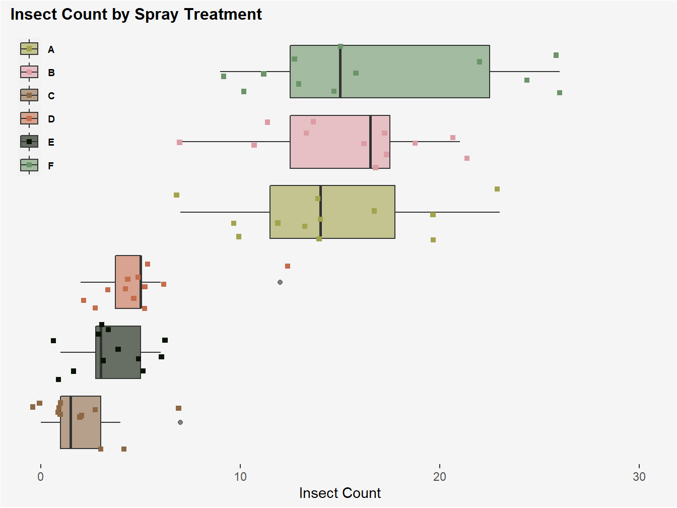
Figure 2.1: Boxplot showing differences and variation in count response between insecticide treatment groups.
Looking at the produced tibble and box plot, it appears that there is variability in insect count for insect plots exposed to different insecticides. Insect plots exposed to Spray F had the highest count on average (16.7), while insect plots exposed to Spray C had the lowest count on average (2.08). The graph and table also illustrate differences in within treatment group variation for the 6 sprays; the spread of the observations vary between each group. For example, the Spray E group had low variance with a standard deviation of 1.73 insects, while Spray F had high variance with a standard deviation of 6.21 insects.
These initial observations from our data exploration are nice, but the question remains as to whether or not the observed variation in the insect counts is truly due to variation due to spray. The next part of the tutorial will demonstrate two models for our data that will help us answer this question.
2.1 Check-in
Suppose the insect plots in the above experiment were comprised using only one insect species. What is one statistical advantage of doing this?
What is the statistical disadvantage of limiting plots to one type of insect species?
References
Beall, Geoffrey. 1942. “The Transformation of Data from Entomological Field Experiments so That the Analysis of Variance Becomes Applicable.” Biometrika 32 (3/4): 243–62.